


Next: 2.4 Summary and outlook
Up: 2. The Kondo Model
Previous: 2.2.3 Calculation of physical
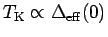
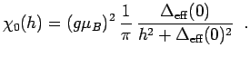
One quantity that can be calculated analytically is the
low-energy limit of the spin
structure factor
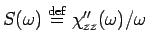 ,
,
 |
(2.20) |
For a vanishing local magnetic field  is just the spin relaxation rate accessible
in e.g. spin resonance experiments.
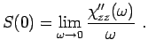
With the result for
is just the spin relaxation rate accessible
in e.g. spin resonance experiments.
With the result for
 from (2.19) we obtain
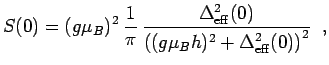 |
(2.21) |
which leads to the curve shown in Fig. 2.2.
Eq. (2.21) is of particular importance because
it explicitly demonstrates
universality,
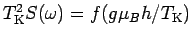 , and allows to directly fit
e.g. experimental data from ESR or NMR experiments and extract the Kondo
, and allows to directly fit
e.g. experimental data from ESR or NMR experiments and extract the Kondo
Figure 2.2:
Universal curve for as function of the local magnetic field
 .
.
|
|
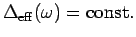
temperature. Note furthermore that the result (2.21) is not
only valid in the Kondo limit, but also holds at the Toulouse point
of the anisotropic Kondo model and everywhere in between. Since it does not
depend on the details of
 it will also be true
for general band structures
it will also be true
for general band structures
 in (2.1) and thus
is eventually the result for in DMFT calculations.
in (2.1) and thus
is eventually the result for in DMFT calculations.
The full frequency dependent
has to be calculated numerically using the
form of the effective hybridization function in Fig. 2.1.
The results for three values of the external field,  ,
,
 and
and
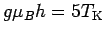
Figure 2.3:
for three characteristic local magnetic fields
,
and
.
|
|
are displayed in Fig. 2.3. These correlation functions provide
a good example for
the usefulness of our mapping to the effective RLM since one can directly
interpret the structures and their frequency and field dependencies in terms of
analytical formulas derived for the RLM. E.g. the high-frequency behavior
of
follows directly from equ. (2.19)
and the behavior of the effective hybridization function
at large energies (which is linear with logarithmic
corrections, see Fig. 2.1):
decays like
 with logarithmic corrections, in agreement with (expensive)
numerical results (23).
with logarithmic corrections, in agreement with (expensive)
numerical results (23).
For the dependence of the dynamical susceptibility on the local magnetic field
one makes use of the fact that
the local magnetic field corresponds to the
on-site energy in the effective RML. Therefore it is obvious that the observed shift
of the resonance peak in
is due to the shifted center
of the resonant level. Furthermore, the depletion of the maximum value is
related to the decreasing occupation of the resonant level, which corresponds
directly to the increasing local magnetization in the SIKM. At the same
time, one observes a decrease of the total spectral weight in
,
which can be accounted for by a transfer to a finite expectation value of
 in the SIKM. There is, however, also a non-trivial effect,
namely the increasing broadening of the resonance peak with increasing magnetic
field. For a RLM with a constant
such a behavior does
not occur; it is entirely related to the fact that with increasing magnetic
field the system starts to notice the energy dependence of the effective
hybridization.
in the SIKM. There is, however, also a non-trivial effect,
namely the increasing broadening of the resonance peak with increasing magnetic
field. For a RLM with a constant
such a behavior does
not occur; it is entirely related to the fact that with increasing magnetic
field the system starts to notice the energy dependence of the effective
hybridization.
The quantity not yet fixed in our calculation is  , or more
precisely the proportionality constant in
, or more
precisely the proportionality constant in
 .
This can most conveniently be done by using Wilson's definition
of the Kondo temperature(3)
.
This can most conveniently be done by using Wilson's definition
of the Kondo temperature(3)
 |
(2.22) |
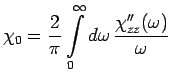
where  is the static magnetic susceptibility
and
is the static magnetic susceptibility
and  the Wilson number.
can be obtained from the imaginary part of the dynamic susceptibility
(2.19) via
the Wilson number.
can be obtained from the imaginary part of the dynamic susceptibility
(2.19) via
 |
(2.23) |
and must in general be evaluated numerically.
At the Toulouse point one can, however, give an analytic answer since
 and thus
 |
(2.24) |
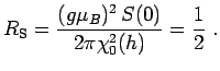
Therefore at the Toulouse point
the Korringa-Shiba relation(24)
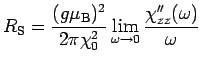 |
(2.25) |
is independent of the local magnetic field
 |
(2.26) |
In the following we will discuss  and the Korringa-Shiba relation
for the Kondo limit
and the Korringa-Shiba relation
for the Kondo limit
 .
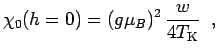
The quantity is particularly convenient for a comparison with NRG results.
.
The quantity is particularly convenient for a comparison with NRG results.
Figure 2.4:
The magnetic susceptibility from equ. (2.23) (circles)
and the same quantity obtained from an NRG calculation.
|
|
In Fig. 3.3 the circles represent the values of
calculated via (2.23) with the effective hybridization function
from Fig. 2.1, and the full line represents the result of an NRG calculation.
We observe excellent agreement for all values of the local magnetic field:
notice that the curves agree without fit parameters.
This example clearly demonstrates
that the nontrivial form of the effective hybridization in
Fig. 2.1 encodes the many-particle physics of the SIKM
in a trivial noninteracting effective model.
The result in Fig. 3.3 can readily be combined with relations
(2.17) and (2.21) to obtain the Wilson ratio(5)
 |
(2.27) |
Our results for the Wilson ratio and the Korringa-Shiba relation obtained
within the effective RLM are collected
in Fig. 2.5.
For the Wilson ratio we would actually have to calculate the quantity
 and not .(5)
However, for the case of small
and not .(5)
However, for the case of small  considered here, both
quantities are equivalent.(25)
One observes that both
considered here, both
quantities are equivalent.(25)
One observes that both  and
and  are independent of the local magnetic
field up to approximately
are independent of the local magnetic
field up to approximately
 , and then start to
Figure 2.5:
Results for the Shiba ratio (full line) and
the Wilson ratio (dashed line) as a function of a local magnetic
field. The
correct limiting values at  are missed by approximately 5%.
|
|
decrease (Shiba ratio), respectively increase (Wilson ratio).
The exact Bethe ansatz solution (4) gives
 independent of the magnetic field strength (see also
Ref. (12)), and local Fermi liquid theory yields
independent of the magnetic field strength (see also
Ref. (12)), and local Fermi liquid theory yields
 for
for
 .(3)
Our limiting values as miss these
exact results by approximately 5%.
Notice that the term
.(3)
Our limiting values as miss these
exact results by approximately 5%.
Notice that the term
 in (2.17)
is very important to obtain this correct value for
in (2.17)
is very important to obtain this correct value for
 .
Remarkably, our simple noninteracting
effective model therefore correctly describes the Wilson ratio in the
Kondo limit (for not too large magnetic fields), which is a hallmark of
strong-coupling Kondo physics.
.
Remarkably, our simple noninteracting
effective model therefore correctly describes the Wilson ratio in the
Kondo limit (for not too large magnetic fields), which is a hallmark of
strong-coupling Kondo physics.
Let us finally analyze the accuracy of our effective model.
Since Fig. 3.3 demonstrates
that integral quantities like are obtained with very good
accuracy for all magnetic fields, one can infer from Fig. 2.5
that quantities depending on low-energy details in frequency
space like
 and are more susceptible to our
approximations for increasing magnetic fields.
This suggests that for such low-energy quantities our effective model
can be employed with very good accuracy (5% error) for magnetic fields below
, and with good accuracy (20% error) still up to approximately
and are more susceptible to our
approximations for increasing magnetic fields.
This suggests that for such low-energy quantities our effective model
can be employed with very good accuracy (5% error) for magnetic fields below
, and with good accuracy (20% error) still up to approximately
 .
.
Next: 2.4 Summary and outlook
Up: 2. The Kondo Model
Previous: 2.2.3 Calculation of physical
© Cyrill Slezak
![\includegraphics[width=0.9\textwidth,clip]{chi0_of_H}](img206.png)
![\includegraphics[width=0.9\textwidth,clip]{Shiba_ed}](img210.png)
![\includegraphics[width=0.9\textwidth,clip]{t1}](img192.png)
![\includegraphics[width=0.9\textwidth,clip]{suscep_i_noNRG}](img194.png)